 |
.gif) |
A Bayesian Networks Approach for Predicting Protein-Protein Interactions from Genomic Data
We have developed an approach using Bayesian networks to predict protein-protein interactions genome-wide in yeast. Our method naturally weights and combines into reliable predictions genomic features only weakly associated with interaction (e.g., messenger RNAcoexpression, coessentiality, and colocalization). In addition to de novo predictions, it can integrate often noisy, experimental interaction data sets. We observe that at given levels of sensitivity, our predictions are more accurate than the existing high-throughput experimental data sets. We validate our predictions with TAP (tandem affinity purification) tagging experiments. Our analysis, which gives a comprehensive view of yeast interactions, is available at genecensus.org/intint. 1 Department of Molecular Biophysics and Biochemistry,
Yale University, 266 Whitney Avenue, Post Office Box 208114, New
Haven, CT 06520, USA.
* Present address:
Computational Biology Center, Memorial Sloan-Kettering
Cancer Center, 307 West 63rd Street, New York, NY 10021,
USA.
Many fundamental biological processes involve protein-protein interactions, and comprehensively identifying them is important to systematically defining their cellular role. New experimental and computational methods have vastly increased the number of known or putative interactions, cataloged in databases (1–7). Much genomic information also relates to interactions indirectly: Interacting proteins are often significantly coexpressed (as shown by microarrays) and colocalized to the same subcellular compartment (8, 9). Unfortunately, interaction data sets are often incomplete
and contradictory (10–12).
In the context of genome-wide analyses, these
inaccuracies are greatly magnified because the protein
pairs that do not interact (negatives) far outnumber those
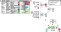
that do (positives). For instance, in yeast, the Consequently, when evaluating protein-protein interactions, one needs to integrate evidence from many different sources (15–17). Here, we propose a Bayesian approach for integrating interaction information that allows for the probabilistic combination of multiple data sets and demonstrate its application to yeast (18). Our approach can be used for combining noisy interaction data sets and for predicting interactions de novo, from other genomic information. The basic idea is to assess each source of evidence for interactions by comparing it against samples of known positives and negatives ("gold-standards"), yielding a statistical reliability. Then, extrapolating genome-wide, we predict the chance of possible interactions for every protein pair by combining each independent evidence source according to its reliability. We verified our predictions by comparing them against existing experimental interaction data (not in the gold-standard) as well as new TAP (tandem affinity purification) tagging experiments. Among the many possible machine-learning approaches that could be applied to predicting interactions (ranging from simple unions and intersections of data sets to neural networks, decision trees, and support-vector machines), Bayesian networks have several advantages (19): They allow for combining highly dissimilar types of data (i.e., numerical and categorical), converting them to a common probabilistic framework, without unnecessary simplification; they readily accommodate missing data; and they naturally weight each information source according to its reliability. In contrast to "black-box" predictors, Bayesian networks are readily interpretable as they represent conditional probability relationships among information sources. The gold-standard data set on which we train ("parameterize") the Bayesian network should ideally be (i) independent from the data sources serving as evidence, (ii) sufficiently large for reliable statistics, and (iii) free of systematic bias. We used the MIPS (Munich Information Center for Protein Sequences) complexes catalog as the gold-standard for positives (6). This hand-curated list of proteincomplexes is based on the literature [8250 pairs in our filtered version (19)]. A negatives gold-standard is harder to define, but essential for successful training. Thus, we synthesized negatives from lists of proteins in separate subcellular compartments (9). Our positive and negative gold-standards satisfy the first two criteria and provide a good practical solution for the third. Hence, our goal, precisely defined, was to predict whether two proteins are in the same complex, not whether they necessarily had direct physical contact. As a measure of reliability, the overlap of information sources (i.e., "interaction data sets," which could either be noisy experimental data or sets of genomic features) with the gold-standards can be expressed in terms of a "likelihood ratio." For example, consider a genomic feature f expressed in binary terms (i.e., "present" or "absent"). The likelihood ratio L(f) is then defined as the fraction of gold-standard positives having feature f divided by the fraction of negatives having f. For two features f1 and f2 with uncorrelated evidence, the likelihood ratio of the combined evidence is simply the product L(f1, f2) = L(f1)L(f2). For correlated evidence, L(f1, f2) cannot be factorized in this way. Bayesian networks are a formal representation of such relationships between features. The combined likelihood ratio is proportional to the estimated odds that two proteins are in the same complex, given multiple sources of information. We predict a protein pair as positive if its combined likelihood ratio exceeds a particular cutoff (L > Lcut) (negative otherwise). To get an overall assessment of how the prediction performs, we segmented the gold-standard into separate training and testing sets (using a sevenfold cross-validation protocol). Then we evaluated the number of true- (TP) and false-positive (FP) predictions in the testing set. Finally, we applied the Bayesian network beyond the testing set, computing likelihood ratios for all possible protein pairs in the genome. Figure 1 schematically shows the information sources and results of our calculations. We term the results "probabilistic interactomes" (PIs), in which each protein pair is associated with a probability measure for being in the same complex (i.e., likelihood ratio L). Our procedure not only allows combining existing experimental interaction data sets (resulting in a PI-experimental or "PIE"), but also the de novo prediction of protein complexes from genomic data sets (when the input data are not interaction data sets per se, resulting in a PI-predicted or "PIP").
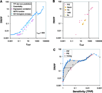
We combined four interaction data sets from high-throughput experiments into the PIE (1–4) (Fig. 1B). The PIE represents a transformation of the individual binary-valued interaction sets into a data set where every protein pair is weighted according to the likelihood that it exists within a complex. We computed the PIP from several genomic data sources: the correlation of mRNA amounts in two expression data sets (one with temporal profiles during the cell cycle, one of expression levels under 300 cellular conditions), two sets of information on biological function, and information about whether proteins are essential for survival (6, 20–22). Although none of these information sources are interaction data per se, they contain information weakly associated with interaction: Two subunits of the same protein complex often have coregulated mRNA expression and similar biological functions and are more likely to be both essential or nonessential (8). For computing the PIE and the PIP, we used two different types of Bayesian networks: a "naïve" network for the PIP and a fully connected one for the PIE (19). The naïve network is simpler to compute but requires information sources with essentially uncorrelated evidence. In contrast, the fully connected Bayesian network accommodates correlated evidence, which is the case for the four experimental interaction data sets. Finally, we combined the PIP, PIE, and gold-standard into a total PI (PIT), which represents our most comprehensive view of the known and putative protein complexes in yeast (23). Because the PIP and PIE data provide essentially uncorrelated evidence for protein-protein interactions, we chose a naïve network to construct the PIT. Figure 1C gives an overview of how we compared the PIP, PIE, gold-standard, and our new experiments. In particular, Fig. 2 shows the performance of the integration resulting in the PIP and PIE. When tested against the gold-standard, we observed that the ratio of true to false positives (TP/FP) increases monotonically with Lcut, confirming L as an appropriate measure of the odds of a real interaction. Conservatively estimated, protein pairs with L > 600 have a better than 50% chance of being in the same complex, suggesting Lcut = 600 as a useful threshold (19). Unless otherwise noted, we use this throughout our analysis. It gives 9897 predicted interactions from the PIP and 163 from the PIE. In contrast, likelihood ratios derived from single genomic features (e.g., mRNA coexpression) or from individual interaction experiments (e.g., the Ho data set) did not exceed the cutoff when used alone, with TP/FP values far below 1. This demonstrates that information sources that, taken alone, are only weak predictors of interactions can yield reliable predictions when combined.
The PIP had a higher sensitivity than the PIE for comparable
TP/FP ratios (Fig.
2C). ("Sensitivity" measures coverage and is defined
as TP/P, where P is the number of gold-standard
positives.) Specifically, the sensitivity of the PIP is
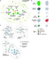
One might ask whether simpler voting procedures can match the performance of more complicated machine-learning methods such as Bayesian networks. To test this hypothesis, we compared the PIP with a voting procedure where each of the four genomic features contributes an additive vote toward positive classification. We found that the Bayesian network achieved greater sensitivity for comparable TP/FP ratios (Fig. 2C) (19). Figure 3 shows parts of the PIP and PIE graphs and how these compare with the gold-standard and our new experiments. First, to test whether the thresholded PIP was biased toward certain complexes, we looked at the distribution of predictions among gold-standard positives (Fig. 3A); they were roughly equally apportioned among the different complexes, suggesting a lack of bias.
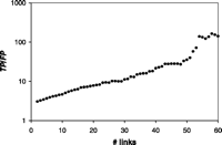
We have thus far treated all interactions as independent. However, the joint distribution of interactions in the PIs can help identify large complexes: An ideal complex should be a "clique" in an interaction graph (i.e., a subgraph with N(N – 1)/2 links between N proteins). Although this rarely happens in practice, because of incorrect or missing links, large complexes tend to have many interconnections within them, whereas false-positive links to outside proteins tend to occur randomly, without a coherent pattern (Fig. 4).
Figure
3B shows parts of the thresholded PIP that are restricted
to proteins with To further test the predictions in the PIP, we conducted TAP-tagging experiments, in which a protein expressed at its normal intracellular concentration ("bait") is tagged and used to "pull down" endogenous protein complexes. We picked 98 proteins as TAP-tagging baits. These produced 424 experimental interactions overlapping with the PIP thresholded at Lcut = 300. (Of these, 185, in turn, overlapped with gold-standard positives, and 16 with negatives, highlighting the reliability of our experiments.) Figure 3C shows three examples of the overlap between the PIP and TAP-tagging. We predicted that the putative DEAD-box RNA helicase Dbp3 interacts with three other RNA helicases (Hca4, Mak5, and Dbp7), with proteins implicated in ribosomal RNA (rRNA) metabolism (e.g., Nop2, Rrp5, Mak5, and components of RNA polymerase I), and with Nsr1, the yeast homolog of mammalian Nucleolin and a GAR domain–containing protein (24). When Dbp3 was TAP-tagged and purified, we found previously unknown interactions with Nsr1, Hca4, and Nop1, connecting Dbp3 with known rRNA-processing proteins. Further purifications with TAP-tagged versions of Mak5, Rrp5, Dbp7, Dbp3, Nsr1, Hca4, and Nop2 verified the physical association. The nucleosome, a fundamental unit within chromatin, provides a second example of overlap. It is composed of eight histones (two H2A, two H2B, two H3, and two H4), which can block RNA polymerase II progression. This blockage is relieved upon interaction with the FACT complex (also known as SPN or yFACT), which consists of Spt16 and Pob3 in yeast. Mammalian Pob3 has a high mobility group (HMG) domain for interaction with histones; however, yeast Pob3 lacks this domain. Instead, the HMG protein Nhp6 (with two virtually identical isoforms, Nhp6A and Nhp6B) binds histones (25–27). [Nhp6 also binds DNA in competition with the nucleosome (28).] Our thresholded PIP and experimental data document a specific interaction between Nhp6A and Hhf1 (H4), pinpointing the contact between the nucleosome and Nhp6 to the H3-H4 heterodimer (Hhf1 and Hht1). This is plausible; because Nhp6 has been shown not to influence nucleosome reassembly (29), it is unlikely that it binds with the H2A-H2B dimer, which needs to reassociate with the nucleosome after binding FACT. The replication complex, a third experimental validation of
the PIP, assembles and dissembles from transiently
interacting subcomplexes (e.g., MCM proteins, ORC, and
polymerases) throughout the cell cycle (8,
30).
Our predicted and experimentally verified interactions
connect it, probably transiently, to another subcomplex,
replication factor A (RFA, composed of Rfa1, Rfa2, and
Rfa3). Specifically, we predicted and verified
interactions between RFA and two proteins associated with
other replication subcomplexes: Rfa2 with Top2 (a
component of the nuclear synaptonemal complex) and Rfa1
with Pri2 (DNA polymerase Finally, we predicted and verified by TAP-tagging that two
proteins involved in translation elongation (Tef2 and
Eft2) interact. This is plausible given that protein
elongation is mediated by three factors in yeast:
EF-1 In summary, we have developed a Bayesian approach for integrating weakly predictive genomic features into reliable predictions of protein-protein interactions. Our de novo prediction of complexes replicated interactions found in the gold-standard positives and PIE. In addition, we confirmed several of our predictions with new experiments. The accuracy of the PIP was comparable to that of the PIE while simultaneously achieving greater coverage. Our procedure lends itself naturally to the addition of more features, possibly further improving results. We anticipate that protein-protein interactions in organisms other than yeast can be explored in similar ways.
Supporting Online Material www.sciencemag.org/cgi/content/full/302/5644/449/DC1 Materials and Methods Figs. S1 to S3 Tables S1 and S2 References 29 May 2003; accepted 29 August
2003
Volume 302, Number 5644, Issue of 17 Oct 2003, pp. 449-453. Copyright © 2003 by The American Association for the Advancement of Science. All rights reserved. |
| ||
.gif) To whom correspondence should be addressed. E-mail:
To whom correspondence should be addressed. E-mail:
 6000 proteins allow
for


 20 links. (Left)
Overlapping gold-standard positives are shown in green, PIE
links in blue, and overlaps with both the PIE and
gold-standard positives in black. (Right) Overlapping
gold-standard negatives are shown in red. Regions with many
red links indicate potential false-positive predictions.
(C) Three PIP complexes that we partially verified by
TAP-tagging. Each complex contains the proteins linked to a
central protein (gray) after thresholding the PIP at
Lcut = 300. Interactions verified by our
TAP-tagging are shown in dark blue and PIE links in light
blue; gray links indicate where TAP-tagging overlapped with
PIE links.
 –primase subunit).
.gif)
.gif)